On “hat algebra”

This post is about “hat algebra” in international trade theory. Non-economists won’t find it interesting.

What is “hat algebra”?

Alan Deardorff’s Glossary of International Economics defines “hat algebra” as

The Jones (1965) technique for comparative static analysis in trade models. Totally differentiating a model in logarithms of variables yields a linear system relating small proportional changes (denoted by carats (^), or “hats”) via elasticities and shares. (As published it used *, not ^, due to typographical constraints.)

The Jones and Neary (1980) handbook chapter calls it a circumflex, not a hat, when explaining its use in proving the Stolper-Samuelson theorem:

a given proportional change in commodity prices gives rise to a greater proportional change in factor prices, such that one factor price unambiguously rises and the other falls relative to both commodity prices… the changes in the unit cost and hence in the price of each commodity must be a weighted average of the changes in the two factor prices (where the weights are the distributive shares of the two factors in the sector concerned and a circumflex denotes a proportional change)… Since each commodity price change is bounded by the changes in both factor prices, the Stolper-Samuelson theorem follows immediately.

I’m not sure when “hat algebra” entered the lexicon, but by 1983 Brecher and Feenstra were writing “Eq. (20) may be obtained directly from the familiar ‘hat’ algebra of Jones (1965)”.

What is “exact hat algebra”?

Nowadays, trade economists utter the phrase “exact hat algebra” a lot. What do they mean? Dekle, Eaton, and Kortum (2008) describe a procedure:

Rather than estimating such a model in terms of levels, we specify the model in terms of changes from the current equilibrium. This approach allows us to calibrate the model from existing data on production and trade shares. We thereby finesse having to assemble proxies for bilateral resistance (for example, distance, common language, etc.) or inferring parameters of technology.

Here’s a simple example of the approach. Let’s do a trade-cost counterfactual in an Armington model with labor endowment $L$ , productivity shifter $\chi$ , trade costs $\tau$ , and trade elasticity $\epsilon$ . The endogenous variables are wage $w$ , income $Y = w \cdot L$ , and trade flows $X_{ij}$ . The two relevant equations are the market-clearing condition and the gravity equation.

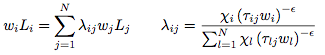
Suppose trade costs change from $\tau_{ij}$ to $\tau'_{ij}$ , a shock $\hat{\tau}_{ij} \equiv \frac{\tau'_{ij}}{\tau_{ij}}$ . By assumption, $\hat{\chi}=\hat{L}=1$ . We’ll solve for the endogenous variables $\hat{\lambda}_{ij}, \hat{X}_{ij}$ and $\hat{w}_{i}$ . Define “sales shares” by $\gamma_{ij}\equiv\frac{X_{ij}}{Y_{i}}$ . Algebraic manipulations deliver a “hat form” of the market-clearing condition.

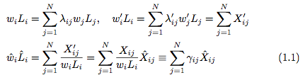
Similarly, let’s obtain “”hat form” of the gravity equation.

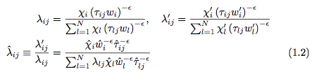
Combining equations (1.1) and (1.2) under the assumptions that $\hat{Y}_{i}=\hat{X}_{i}$ and $\hat{\chi}=\hat{L}=1$ , we obtain a system of equations characterizing an equilibrium $\hat{w}_i$ as a function of trade-cost shocks $\hat{\tau}_{ij}$ , initial equilibrium shares $\lambda_{ij}$ , and $\gamma_{ij}$ , and the trade elasticity $\epsilon$ :

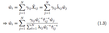
If we use data to pin down $\epsilon, \lambda_{ij}$ , and $\gamma_{ij}$ , then we can feed in trade-cost shocks $\hat{\tau}$ and solve for $\hat{w}$ to compute the predicted responses of $\lambda'_{ij}$ .

Why is this “exact hat algebra”? When introducing material like that above, Costinot and Rodriguez-Clare (2014) say:

We refer to this approach popularized by Dekle et al. (2008) as “exact hat algebra.”… One can think of this approach as an “exact” version of Jones’s hat algebra for reasons that will be clear in a moment.

What is “calibrated share form”?

Dekle, Eaton, and Kortum (AERPP 2007, p.353-354; IMF Staff Papers 2008, p.522-527) derive the “exact hat algebra” results without reference to any prior work. Presumably, Dekle, Eaton, and Kortum independently derived their approach without realizing a connection to techniques used previously in the computable general equilibrium (CGE) literature. The CGE folks call it “calibrated share form”, as noted by Ralph Ossa and Dave Donaldson.

A 1995 note by Thomas Rutherford outlines the procedure:

In most large-scale applied general equilibrium models, we have many function parameters to specify with relative ly few observations. The conventional approach is to calibrate functional parameters to a single benchmark equilibrium… Calibration formulae for CES functions are messy and difficult to remember. Consequently, the specification of function coefficients is complicated and error-prone. For applied work using calibrated functions, it is much easier to use the “calibrated share form” of the CES function. In the calibrated form, the cost and demand functions explicitly incorporate

benchmark factor demands

benchmark factor prices

the elasticity of substitution

benchmark cost

benchmark output

benchmark value shares

Rutherford shows that the CES production function $y(K,L) = \gamma \left(\alpha K^{\rho} + (1-\alpha)L^{\rho}\right)^{1/\rho}$ can be calibrated relative to a benchmark with output $\bar{y}$ , capital $\bar{K}$ , and labor $\bar{L}$ as $y = \bar{y} \left[\theta \left(\frac{K}{\bar{K}}\right)^{\rho} + (1-\theta)\left(\frac{L}{\bar{L}}\right)^{\rho}\right]^{1/\rho}$ , where $\theta$ is the capital share of factor income. If we introduce “hat notation” with $\hat{y} = y/\bar{y}$ , we get $\hat{y} = \left[\theta \hat{K}^{\rho} + (1-\theta)\hat{L}^{\rho}\right]^{1/\rho}$ . Similar manipulations of the rest of the equations in the model delivers a means of computing counterfactuals in the CGE setting.